Data Structures + Algorithms = Programs
Recursion: When you defined something in terms of itself.
a function that referese to itself inside it's fucntion
Good for tasks that have repeated subtasks, eg sorting and searching
Recursion can cause stack overflow
3 steps
counter = 0
def inception():
    global counter
    print(counter, end=" ")
    if counter > 3:
        return "Done!" #base case
    counter += 1
    return inception() #recursive case
inception()
0 1 2 3 4
'Done!'
def factorial(num):
    if (num < 1):
        return 1
    return num * factorial(num - 1)
factorial(5)
# O(n)
120
def fibonacci(num):
    if num < 2:
        return num
    return fibonacci(num-1) + fibonacci(num-2)
fibonacci(10)
# O(2^n)
55
def reverseString(str) :
    if len(str) < 1:
        return ""
    return reverseString(str[1:]) + str[0]
reverseString('yoyo mastery')
'yretsam oyoy'
Anything that can be done recursivly can be done iteratively
Recursion can help the code be dry and more readable
Recursion are best for searching and sorting in trees
Tail recursion is a recursion that each stack is indepent, and does not rely on the response of the calling self.
If the programming language engine supports tail recurssion, it can have a space big o of 1.
Because the engine would remove the stack after it sees that it no longer it needs it.
But tail recursions are harder to implement, and rarely supported.
def tail_factorial(num,total):
    if (num == 0):
        return total
    return tail_factorial(num -1,total*num)

tail_factorial(4,1)
24
2 Types:
Comparison sort
Non-Comparsion Sort
Each pair compare to each other, the bigger one will be passed and it continue for the rest
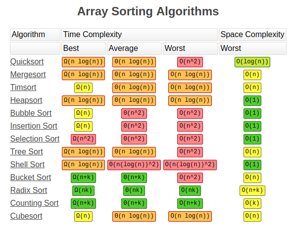
Time Complexity Big O of n^2
Space Complexity Big O of 1
Usage: Rarely used, more educational aspects
def bubbleSort(lst):
    length = len(lst) - 1
    for a in range(length):
        for b in range(length):
            if lst[b] > lst[b+1]:
                lst[b], lst[b+1] = lst[b+1], lst[b]
    return lst
bubbleSort([99,44,6,2,1,5,63,87,283,4,0])
[0, 1, 2, 4, 5, 6, 44, 63, 87, 99, 283]
Goes through the list and mark the lowest value and bring it to beginning, and repeat
Time Complexity Big O of n^2
Space Complexity Big O of 1
Usage: Mostly used for teaching purposes
def selectionSort(lst):
    length = len(lst)
    for a in range(length):
        index = a
        lowest = lst[a]
        for b in range(a+1,length):
            if lowest > lst[b]:
                lowest = lst[b]
                index = b
        lst[a] , lst[index] = lst[index] , lst[a]
    return lst
selectionSort([99,44,6,2,1,5,63,87,283,4,0])
[0, 1, 2, 4, 5, 6, 44, 63, 87, 99, 283]
Time Complexity Big O of n^2
Space Complexity Big O of 1
best algorithm for nearly sorted lists
Usage: Small list
def insertionSort(lst):
    length = len(lst)
    for b in range(1,length):
        if lst[b] <= lst[0]:
            temp = lst[b]
            del lst[b]
            lst = [temp]+lst[:]
        elif lst[b] >= lst[b-1]:
            pass
        else:
            for i in range(b):
                if lst[b] < lst[i]:
                    temp = lst[b]
                    del lst[b]
                    lst = lst[:i]+[temp]+lst[i:]
    return lst
insertionSort([99,44,6,2,1,5,63,87,283,4,0])
[0, 1, 2, 4, 5, 6, 44, 63, 87, 99, 283]
Time Complexity Big O of n log n
Space Complexity Big O of n
uses divide and conquer method
Usage: For huge files that can be stored in memory
def merge(left,right):
    result = []
    leftIndex = 0
    rightIndex = 0
    while leftIndex < len(left) and rightIndex < len(right):
        if left[leftIndex] < right[rightIndex]:
            result.append(left[leftIndex])
            leftIndex +=1
        else:
            result.append(right[rightIndex])
            rightIndex+=1
    return result+left[leftIndex:]+right[rightIndex:];

def mergeSort(lst):
    if len(lst) == 1:
        return lst
    mid = len(lst)//2
    return merge(mergeSort(lst[:mid]),mergeSort(lst[mid:]))

mergeSort([99,44,6,2,1,5,63,87,283,4,0])
[0, 1, 2, 4, 5, 6, 44, 63, 87, 99, 283]
Time Complexity Big O of n log n (worst case O(n^2) if pivot is the smallest or the largest)
Space Complexity Big O of log n
uses divide and conquer method
Usage: Most popular algorithm, but the worst case is very expensive
#My version
def quickSort(lst):
    if len(lst) == 2:
        if lst[0] > lst[1]:
            return [lst[1],lst[0]]
        else:
            return lst
    elif len(lst) <= 1:
        return lst
    #divide
    pivot = lst[len(lst)-1]
    left = []
    right = []
    for i in range(len(lst)-1):#if pivot is not the last item,
        #here should change to len(lst),
        #and the iteration which the count is same as pivot should be skipped
        if lst[i] < pivot:
            left.append(lst[i])
        else:
            right.append(lst[i])
    return quickSort(left) + [pivot] + quickSort(right)

quickSort([99,44,6,2,1,5,63,87,283,4,0])
[0, 1, 2, 4, 5, 6, 44, 63, 87, 99, 283]
# Given algorithm
def swap(array, firstIndex, secondIndex):
    array[firstIndex], array[secondIndex] = array[secondIndex], array[firstIndex]

def partition(array, pivot, left, right):
    pivotValue = array[pivot]
    partitionIndex = left
    for i in range(left,right):
        if array[i] < pivotValue:
            swap(array, i, partitionIndex)
            partitionIndex+=1
    swap(array, right, partitionIndex)
    return partitionIndex

def quickSort(array, left, right):
    if left < right :
        pivot = right
        partitionIndex = partition(array, pivot, left, right)
        #sort left and right
        quickSort(array, left, partitionIndex - 1)
        quickSort(array, partitionIndex + 1, right)
    return array


#Select first and last index as 2nd and 3rd parameters
numbers = [99, 44, 6, 2, 1, 5, 63, 87, 283, 4, 0]
quickSort(numbers, 0, len(numbers)- 1)
print(numbers)
[0, 1, 2, 4, 5, 6, 44, 63, 87, 99, 283]
Timsort is a hybrid stable sorting algorithm, derived from merge sort and insertion sort, designed to perform well on many kinds of real-world data. It was implemented by Tim Peters in 2002 for use in the Python programming language. The algorithm finds subsequences of the data that are already ordered (runs) and uses them to sort the remainder more efficiently. This is done by merging runs until certain criteria are fulfilled
Time Complexity Big O of n log n
Space Complexity Big O of n
uses a hybrid of merge and isertion sort
Usage: Python's default sort algorithm
MIN_MERGE = 32

def calcMinRun(n):
    r = 0
    while n >= MIN_MERGE:
        r |= n & 1
        n >>= 1
    return n + r

def insertionSort(arr, left, right):
    for i in range(left + 1, right + 1):
        j = i
        while j > left and arr[j] < arr[j - 1]:
            arr[j], arr[j - 1] = arr[j - 1], arr[j]
            j -= 1

def merge(arr, l, m, r):
    len1, len2 = m - l + 1, r - m
    left, right = [], []
    for i in range(0, len1):
        left.append(arr[l + i])
    for i in range(0, len2):
        right.append(arr[m + 1 + i])
    i, j, k = 0, 0, l
    while i < len1 and j < len2:
        if left[i] <= right[j]:
            arr[k] = left[i]
            i += 1
        else:
            arr[k] = right[j]
            j += 1
        k += 1
    while i < len1:
        arr[k] = left[i]
        k += 1
        i += 1
    while j < len2:
        arr[k] = right[j]
        k += 1
        j += 1

def timSort(arr):
    n = len(arr)
    minRun = calcMinRun(n)
    for start in range(0, n, minRun):
        end = min(start + minRun - 1, n - 1)
        insertionSort(arr, start, end)
    size = minRun
    while size < n:
        for left in range(0, n, 2 * size):
            mid = min(n - 1, left + size - 1)
            right = min((left + 2 * size - 1), (n - 1))
            if mid < right:
                merge(arr, left, mid, right)
        size = 2 * size
This sort algorithm is used for Directed Acylic Graphs (DAG)
It sorts nodes with least Indegrees to the most
Indegree: indegrees are the incoming vertexes to each node
How this works is that it first create an indegree list for all nodes. Then we start by removing nodes which have an indegree of 0. When removing a node we should also reduce the indegree of all other nodes depending on that. We keep going till all nodes have reach indegree of zero and removed.
Warning: if the graph is not acylic (there is a loop in it) we won't be able to remove all nodes.
This can also be used to see if there is a loop in a graph

edges = [[1,0],[2,1],[2,5],[0,3],[4,3],[3,5],[4,5]]
def topologicalSort(numCourses, prerequisites):
    lst = [[] for i in range(numCourses)]
    indegree = [0 for i in range(numCourses)]
    for pair in prerequisites:
        lst[pair[1]].append(pair[0])
        indegree[pair[0]]+= 1

    print("Adjacent List: ", lst)
    print("Indegrees:     ", indegree)
    sortedList = []

    stack = [a for a,b in enumerate(indegree) if b == 0]
    while stack:
        v, stack = stack[0],stack[1:]
        sortedList.append(v)
        for i in lst[v]:
            if (indegree[i]-1 == 0):
                stack.append(i)
            indegree[i] -= 1
    return sortedList
topologicalSort(6, edges)
Adjacent List:  [[1], [2], [], [0, 4], [], [2, 3, 4]]
Indegrees:      [1, 1, 2, 1, 2, 0]
[5, 3, 0, 4, 1, 2]
Choosing a the most proper sorting algorithm for the following cases:
1 - Sort 10 schools around your house by distance: insertion sort
2 - eBay sorts listings by the current Bid amount: radix or counting sort
3 - Sport scores on ESPN: quick sort
4 - Massive database (can't fit all into memory) needs to sort through past year's user data: merge sort
5 - Almost sorted Udemy review data needs to update and add 2 new reviews: insertion sort
6 - Temperature Records for the past 50 years in Canada: radix or counting quick or sort insertion
7 - Large user name database needs to be sorted. Data is very random.: merge or quick sort
8 - You want to teach sorting for the first time: Bubble, selection sort
Sequentially goes through items can compare each item with the searching value
Time Complexity of big O of n
def linearSearch(lst,value):
    for i in lst:
        if i == value:
            return True
    return False
linearSearch([99,44,6,2,1,5,63,87,283,4,0], 5)
True
requires a sorted list
Time Complexity of big O of log n
def binarySearch(arr, x):
    low = 0
    high = len(arr) - 1
    mid = 0
    while low <= high:
        mid = (high + low) // 2
        if arr[mid] < x:
            low = mid + 1 #ignore left half
        elif arr[mid] > x:
            high = mid - 1 # ignore right half
        else:
            return mid
    return -1

binarySearch([0, 1, 2, 4, 5, 6, 44, 63, 87, 99, 283], 5)
4
# binary tree code for following topic
class Node:
    def __init__(self,value):
        self.left = None
        self.right = None
        self.value = value
class BinaryTree:
    def __init__(self):
        self.root = None

    def insert(self, value):
        leaf = Node(value)
        if not self.root:
            self.root = leaf
            return
        node = self.root
        while node:
            temp = node
            if leaf.value < node.value:
                node = node.left
                if not node:
                    temp.left = leaf
            else:
                node = node.right
                if not node:
                    temp.right = leaf

    #divid and conquer
    def lookup(self,value):
        if self.root.value == value:
            return True
        node = self.root
        while node:
            if value < node.value:
                node = node.left
            elif value == node.value:
                return True
            else:
                node = node.right
        return False

    def bfs(self):
        currentNode = self.root
        lst = []
        queue = []
        queue.append(currentNode)

        while len(queue) > 0:
            currentNode = queue[0] #shift
            queue = queue[1:]
            lst.append(currentNode.value)
            if currentNode.left:
                queue.append (currentNode.left)
            if currentNode.right:
                queue.append (currentNode.right)
        return lst

    def dfs(self,node,lst):
        if node == None:
            return
        lst.append(node.value) #lst here for pre order
        self.dfs(node.left, lst)
        #lst here for in order
        self.dfs(node.right, lst)
        #lst here for post order
        return lst

    def dfsInorderIterative(self):
        lst = []
        stack = []
        node = self.root
        while stack or node is not None:
            if node is not None:
                stack.append(node)
                node = node.left
            else:
                node = stack.pop()
                lst.append(node.value)
                node = node.right
        return lst


"""
     9
   /   \
  4     20
 / \   /  \
1   6 15  170
"""
tree = BinaryTree()
tree.insert(9)
tree.insert(4)
tree.insert(6)
tree.insert(20)
tree.insert(170)
tree.insert(15)
tree.insert(1)

print(tree.bfs())
print(tree.dfs(tree.root,[]))
print(tree.dfsInorderIterative())
[9, 4, 20, 1, 6, 15, 170]
[9, 4, 1, 6, 20, 15, 170]
[1, 4, 6, 9, 15, 20, 170]
Time Complexity of big O of n
for graph traversal
goes down through the tree level by level
for previous tree the order would be: 9 4 20 1 6 15 170
Cons:
Shortest path
Closer nodest
Prons:
More Memory
def breadthFirstSearch(queue, value):
    if len(queue) < 1:
        return False
    currentNode = queue.pop()
    if currentNode.value == value:
        return True
    if currentNode.left:
        queue.append (currentNode.left)
    if currentNode.right:
        queue.append (currentNode.right)
    return breadthFirstSearch(queue, value)

breadthFirstSearch([tree.root],15)
True
array = [
    [1, 2, 3, 4, 5 ],
    [6, 7, 8, 9, 10],
    [11,12,13,14,15],
    [16,17,18,19,20],
]

def dfs_2D_array_search(matrix):
    # DFS Directions
    directions = [
    (-1,0), #up
    (0, 1), #right
    (1, 0), #down
    (0,-1)  #left
    ]
    #this creates a 2D replica of the matrix with only false boolean values
    """
    [[F, F, F, F, F],
     [F, F, F, F, F],
     [F, F, F, F, F],
     [F, F, F, F, F]]
    """
    seen = [ [False for j in range(len(matrix[0]))] for i in range(len(matrix))]
    values = []
    def dfs(matrix,row,col,seen,val):
        if row < 0 or col < 0 or row >= len(matrix) or col >= len(matrix[0]) or seen[row][col]:
            return
        seen[row][col] = True
        val.append(matrix[row][col])
        for i,j in directions:
            dfs(matrix,row+i,col+j,seen,values)
    dfs(matrix,0,0,seen,values)
    return values

dfs_2D_array_search(array)
[1, 2, 3, 4, 5, 10, 15, 20, 19, 14, 9, 8, 13, 18, 17, 12, 7, 6, 11, 16]
adjList = [[1,3], [0],[3,8],[0,4,5,2],[3,6],[3],[4,7],[6],[2]]

def graph_bfs(graph):
    queue = [0]
    visited = []
    while queue:
        vertex, queue = queue[0], queue[1:]
        visited.append(vertex)
        for connection in graph[vertex]:
            if connection not in visited:
                queue.append(connection)
    return visited

graph_bfs(adjList)
[0, 1, 3, 4, 5, 2, 6, 8, 7]
Time Complexity of big O of n
for tree traversal
goes down through one branch till there is no more childern, then goes back up and goes to the other childern
for previous tree the order would be: 9 4 1 6 20 15 170
Cons:
Less Memory
Does path exist?
Prons:
can get slow
101
| \
33 105
3 Types:
inorder - 33 101 105 (after left)
preorder 101 33 105 (at beginning)
postorder 33 105 101 (after right)
def depthFirstSearch(node, value):
    if node == None:
        return False

    if node.value == value:
        return True
    if depthFirstSearch(node.left, value):
        return True
    if depthFirstSearch(node.right, value):
        return True
    return False

depthFirstSearch(tree.root,15)
True
array = [
    [1, 2, 3, 4, 5 ],
    [6, 7, 8, 9, 10],
    [11,12,13,14,15],
    [16,17,18,19,20],
]

def bfs_2D_array_search(matrix):
    directions = [
    (-1,0), #up
    (0, 1), #right
    (1, 0), #down
    (0,-1)  #left
    ]
    seen = [ [False for j in range(len(matrix[0]))] for i in range(len(matrix))]
    row,col =len(matrix)//2, len(matrix[0])//2 # middle of the matrix, or start from (0,0)
    values = [matrix[row][col]]
    queue = [(row,col)]
    seen[row][col] = True
    while queue:
        point, queue = queue[0], queue[1:]
        row,col = point
        for i,j in directions:
            if row+i < 0 or col+j < 0 or row+i >= len(matrix) or col+j >= len(matrix[0]) or seen[row+i][col+j]:
                continue
            else:
                seen[row+i][col+j] = True
                values.append(matrix[row+i][col+j])
                queue.append((row+i,col+j))
    return values

bfs_2D_array_search(array)
[13, 8, 14, 18, 12, 3, 9, 7, 15, 19, 17, 11, 4, 2, 10, 6, 20, 16, 5, 1]
adjList = [[1,3], [0],[3,8],[0,4,5,2],[3,6],[3],[4,7],[6],[2]]

def graph_dfs(graph,vertex=0,visited=[]):
    visited.append(vertex)
    for connection in graph[vertex]:
        if connection not in visited:
            graph_dfs(graph,connection,visited)
    return visited

graph_dfs(adjList)
[0, 1, 3, 4, 6, 7, 5, 2, 8]
Choose between BFS and DFS:
If you know a solution is not far from the root of the tree : BFS
If the tree is very deep and solutions are rare : BFS
If the tree is very wide : DFS
If solutions are frequent but located deep in the tree : DFS
Determining whether a path exists between two nodes : DFS
Finding the shortest path : BFS
it is an optimization technique
If you have something you can cache, dynamic programming is the best chioce
A method of solving problems by breaking it down into a collection of sub-problems,
and then solving each of them only once,
and storing their solutions in case next time the same sub-problem occurs
Memoization ~ Caching
# Not using memoization
def addTo80(n):
    print("long time", end=', ')
    return n+80

addTo80(5)
addTo80(5)
addTo80(5)
long time, long time, long time,
85
# Using memoization
cache = {}
def memoizedAddTo80(n):
    global cache
    if n in cache:
        return cache[n]
    print("long time", end=', ')
    cache[n] = n + 80
    return cache[n]
memoizedAddTo80(5)
memoizedAddTo80(5)
memoizedAddTo80(5)
long time,
85
# Using memoization and closure
def memoizer80():
    cache = {}
    def memoizedAddTo80(n):
        if n in cache:
            return cache[n]
        print("long time", end=', ')
        cache[n] = n + 80
        return cache[n]
    return memoizedAddTo80
memoized = memoizer80()
memoized(5)
memoized(5)
memoized(5)
long time,
85
# Fibonacci without memoization
counter = 0
def fibonacci(num):
    global counter
    counter += 1
    if num < 2:
        return num
    return fibonacci(num-1) + fibonacci(num-2)
print(fibonacci(30))
print(counter)
# O(n^2)
832040
2692537
# Fibonacci with memoization
counter = 0
cache = {}
def fibonacci(num):
    global counter, cache
    counter += 1
    if num in cache:
        return cache[num]

    if num < 2:
        return num
    cache[num] = fibonacci(num-1) + fibonacci(num-2)
    return cache[num]

print(fibonacci(30))
print(counter)
# O(n)
832040
59
This method depends on dynamic progamming, and it is used for optimzation problems.
Find the shortest path from one node to the others. This method can handle negative weights, but will not work on a cycle witha a negative weight
N: Number of the nodes, E: the number of the edges
Time: O(N . E)
Space: O(N)
Algorithm:

# [source, target, weight]
weightedEdges = [[1,2,9],[1,4,2],[2,5,1],[4,2,4],[4,5,6],[3,2,3],[5,3,7],[3,1,5]] #n=5 k=1 Exp=14

import math
def bellmanFord(weightedEdges,size, start):
    weights = [ math.inf for i in range(size)]
    weights[start-1] = 0

    for _ in range(size-1):
        changed = False
        for source,target,weight in weightedEdges:
            if weights[source-1] + weight < weights[target-1]:
                weights[target-1] = weights[source-1] + weight
                changed = True
        if not changed:
            break

    return weights

bellmanFord(weightedEdges,5,1)
[0, 6, 14, 2, 7]
Smilar to dynamic programming, but back tracking is used for
In backtracking there can be multiple solutions
There are two steps to backtracking:
For optimazation problems
It is used to find the path with the maximum or minimum value
Greedy method always goes for the biggest/smallest value
A greedy method algorithm, used for optimzation problems.
Find the shortest path from one node to the others.
This method can not handle negative weights, because we do no go back to a vertex once we pass it
N: Number of the nodes, E: the number of the edges
Time: O(N + E Log E)
Space: O(N + E)
Algorithm:

# starting from k, the shortest time it takes to traverse
# [source, target, weight]
import math
weightedEdges = [[1,2,9],[1,4,2],[2,5,1],[4,2,4],[4,5,6],[3,2,3],[5,3,7],[3,1,5]]

def dijkstra(weightedEdges,size, start):
    weights = [ math.inf for i in range(size)]
    adjList = [ [] for i in weights]

    weights[start-1] = 0 #start from 0
    heap = []            #Better if Priority Queue
    heap.append(start-1)

    for i in range(len(weightedEdges)):
        source = weightedEdges[i][0] - 1
        target = weightedEdges[i][1] - 1
        weight = weightedEdges[i][2]
        adjList[source].append((target,weight))
    print("Graph:", adjList)

    while heap:
        currentVertex = min(heap, key=lambda a : weights[a]) #getting the min value
        heap = heap[:heap.index(currentVertex)] + heap[heap.index(currentVertex)+1:] #removing the min value
        adj = adjList[currentVertex]
        for index,weight in adj:
            if weights[currentVertex] + weight < weights[index]:
                weights[index] = weights[currentVertex] + weight
                heap.append(index)

    return weights

dijkstra(weightedEdges,5,1)
Graph: [[(1, 9), (3, 2)], [(4, 1)], [(1, 3), (0, 5)], [(1, 4), (4, 6)], [(2, 7)]]
[0, 6, 14, 2, 7]
We use a hash map with look up of O(n) to store the item we previously have seen
def find_reaccuring(ar):
    hsh = dict()
    for e in ar:
        if e in hsh:
            return e
        hsh[e]=True
    return None
We traverse through an array from both ends till the two pointers reach each other.

def palindromeCheck(st):
    if len(st) <= 1:
        return True
    left = 0
    right = len(st)-1
    while left <= right:
        if st[left] == st[right]:
            left += 1
            right -= 1
        else:
            return False
    return True
sliding window is a sub-list that runs over an underlying collection. I.e., if you have an array like

def longest_substring(st):
    length = len(st)
    if length <= 1:
        return length
    max_count = 0
    left = 0
    cache = {}
    a= 0
    while a < length:
        s = st[a]
        seen = cache[s] if s in cache else -1
        if seen >= left:
            left = seen +1
        cache[s] = a
        max_count = max(max_count, a-left+1)
        a+=1
    return max_count
It is an effient algorithm for cycle detection in Linked List.
Needs 2 pointers. One (Tortoise) which moves at 1 step per iteration,
and Two (Hare) which moves 2 steps per iterations
The moment these two lap on the same node, we know we have a cycle
Then we create 2 new pointers at the begining and at the node where we found we have a cycle
We iterate from each point to the next node by one step till they lap on the same node, that node is where the loop started
def toroiseAndHare(head):
    toroise = head.next
    hare = head.next.next
    isCycle = False
    while hare and hare.next:
        if toroise is hare:
            isCycle = True
            break
        toroise = toroise.next
        hare = hare.next.next
    if isCycle:
        pointer1 = head
        pointer2 = toroise
        while pointer2 is not pointer1:
            pointer2 = pointer2.next
            pointer1 = pointer1.next
        return pointer1.val
    else:
        return False
Solving a problem by splitting it into smaller problems and then solving each of them.
Divide & Conquer must have 3 characteristics:

example:
Andrei Neagoie: Master the Coding Interview: Data Structures + Algorithms
https://academy.zerotomastery.io/p/master-the-coding-interview-data-structures-algorithms
Yihua Zhang: Master the Coding Interview: Big Tech (FAANG) Interviews
https://academy.zerotomastery.io/p/master-the-coding-interview-faang-interview-prep


